INTRODUCTION

Artificial Intelligence

General Definitions and classifications

Artificial Intelligence encompasses a wide variety of types and are classified according to ability or functionality. Ability ranges from task-specific Weak or Narrow AI to the “Hal – type AI from 2001 Space Odyssey” or Super AI which is far more intelligent than humans.

AI based upon Ability

Weak or narrow AI

This type of AI is designed to perform specific tasks, such as speech or facial recognition. Weak AI is already in use today and has proven to be effective.

Strong or General AI

This type of AI can perform any task that a human can, such as thinking, reasoning, and solving puzzles. Strong AI has the potential to revolutionize many aspects of life.

Super AI

This type of AI surpasses human intelligence and can perform tasks better than humans.

AI based upon Functionality

There are several types of artificial intelligence (AI) based upon Functionality, including: ranging from the simplest programming that performs functions mathematically to yield decisions to those works-in-progress that are approaching self-awareness.

Reactive Machines

The oldest form of AI – reactive machines only use current data to make decisions and don’t store past memories or data.  These machines are hardly “intelligent” at all because no training or learning was required – only programming. Many early products associated with medical data sorting and presentation software are referred to as AI but add no additional information resulting from machine learning. An example of this radiologic display software is the Philips DynaCAD Prostate system (Philips Medical Systems, Netherlands).
ited Memory.

Limited Memory

This is the most common type of AI today, and it learns from past experiences and observations to build knowledge. It uses historical data and pre-programmed information to make predictions and perform complex tasks.
Subsets of this class include Generative and Regenerative AI.ited Memory.

Generative AI: Creates new content, such as images, text, and music, from scratch or based on a text prompt. It can be used to enhance human capabilities in creative and professional fields, such as marketing, entertainment, and customer service. For example, generative AI can design personalized treatment plans for patients based on their data.

Regenerative AI: Builds on generative AI’s foundation to create systems that improve and sustain ecosystems and communities. It focuses on principles of regeneration, such as restoring, renewing, and growing systems, to ensure that AI applications contribute to the health of the planet and societies. For example, regenerative AI can adapt treatment plans in real-time as new information becomes available, such as changes in a patient’s condition or new medical research findings. It can also evolve city planning models to reflect changing demographics, economic conditions, and environmental factors. Limited Memory.

Theory of Mind

Theory of mind AI is the ability of artificial intelligence (AI) to understand and model the thoughts, intentions, and emotions of other agents, such as humans or other AI. This capability is important for effective communication and social interaction, as it implies an understanding of the perspectives and beliefs of other entities.
Some examples of theory of mind scenarios include: Detecting an indirect request, Detecting a false belief, and Detecting faux pas.

Self-aware AI

This type of AI is still in the planning stages, and developers are trying to create a conscious side to machines.
Conclusion: Be aware of the use of AI in marketing literature as distinction is seldom made by vendors claiming AI when no machine learning was involved intelligence added. In contrast, AI that interprets medical images and detects pathologies would be considered General/Strong AI with Limited Memory.

Classification Types of Machine Learning

The next questions we address are what are the various types of machine learning systems.

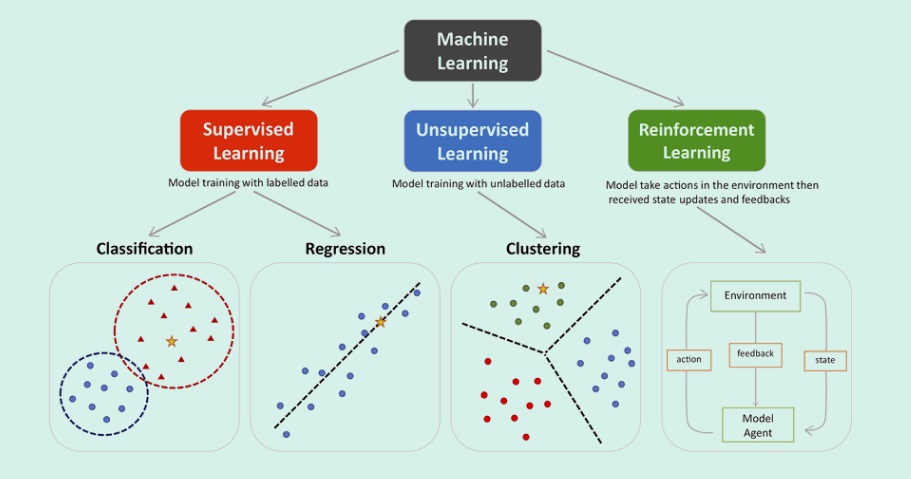
Machine learning encompasses three main types -supervised, unsupervised, and reinforcement. Supervised learning involves classification and regression, where models are trained with labeled data such as MRI image sets with labeled or manually segmented organs and pathologies within. Unsupervised learning focuses on clustering and finding patterns in unlabeled data such as might be found in remote sensing or photographic analyses seeking specific groups. Reinforcement learning improves model performance through interaction with the environment. In the provided visualization, colored dots and triangles represent training data, while yellow stars symbolize new data that can be predicted by the trained model.

We’ll focus on Supervised Learning as this is the type of learning used in training General/Limited memory AI employed in Medical Imaging analyses software such as cancer detection in MR images.

Classification type machines utilize Support Vector, decision trees or random forest algorithms.

A support vector machine (SVM) is a supervised machine learning algorithm that uses an n-dimensional space to classify data by finding a function that separates data by levels of a categorical variable. SVMs are often used to solve classification problems, especially binary classification problems, which require classifying data into two groups.

SVMs work by:

    1. Transforming input data into a higher-dimensional feature space
    2. Finding an optimal line or hyperplane that maximizes the distance between each class in the space
    3. Drawing a decision boundary, also known as a hyperplane, near the extreme points in the data set

SVMs are highly accurate at modeling complex decision boundaries with less overfitting than other methods. In the sample image below, a linear regression is shown where the maximum-minimum hyperplan and margins for an SVM trained with samples from two classes. Samples on the margin are called the support vectors.

Decision Tree machines

Decision Tree machines are a type of supervised learning algorithm in machine learning that use a tree-like structure to categorize or make predictions based on how a set of questions were answered. They are named for their upside-down tree shape, which has a root node, branches, internal nodes, and leaf nodes.
Decision trees are used for classification and regression modeling:

Classification trees
Determine if an event happened or not, usually with a “yes” or “no” outcome. For example, a decision tree could be used to accept or deny credit applicants based on data like credit score, debt burden, and length of credit history.

Decision trees use a divide and conquer strategy to identify the best split points within the tree, repeating the process in a top-down manner until all records have been classified. The root node starts with a specific question of data, and the branches hold potential answers. The nodes resulting from the splitting of the root node are called decision nodes, which represent intermediate decisions or conditions. The nodes where further splitting is not possible are called leaf nodes, or terminal nodes, and often indicate the final classification or outcome.

Decision trees are popular in machine learning because they are a simple way to structure a model and understand the model’s decision-making process.

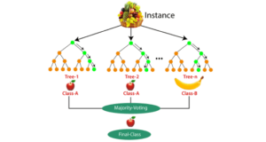
Random forest (RF) is a machine learning algorithm that combines the results of multiple decision trees to produce a single result. It’s a supervised algorithm that can be used for both classification and regression problems. RFs are the most popular type of decision tree ensemble and are known for being flexible, easy to use, and powerful.

RFs use two sources of randomness to ensure that the decision trees are relatively independent:

Bagging
Each decision tree is trained on a random subset of the training set examples, with replacement. This approach is often used to reduce variance in noisy datasets.

Attribute sampling
At each node, only a random subset of features are tested as potential splitters.
To build each tree, RFs also perturb the data set by bootstrapping, which means randomly sampling members of the original data set with replacement. This results in a data set that is the same size as the original, but with a constantly changing version of the data. Each subset, or “bootstrap sample”, may have some data points that appear multiple times, while others may not appear at all.

When making predictions, each tree in the RF votes for a single class, and the RF prediction is the class that receives the most votes. For example, in regression, each tree predicts the value of y for a new data point, and the RF prediction is the average of all of the predicted values.

RFs are used in many different fields, including banking, the stock market, medicine, e-commerce, and finance. However, they do have some disadvantages, such as becoming too slow and ineffective for real-time predictions if there are too many trees. Increased accuracy also requires more trees, which can slow down the model further.
Regression type machines utilize Linear Regression, Neural Network Regression or Support Vector Regression.

Linear Regression
Linear Regression is a statistical technique used in machine learning to find the relationship between variables, or features and a label. It’s a supervised learning algorithm that models a dependent variable as a function of independent variables by finding a line that best fits the data. The line can then be used to make predictions for continuous or numeric variables.

For example, linear regression can be used to predict the price of a house based on the number of rooms it has, or to predict weight based on height and age. In these examples, the dependent variable is the price or weight, and the independent variables are the number of rooms, height, and age.

Linear regression is advantageous when there are at least two variables in the data. It’s used in many fields, including business, science, and data science, to convert data into insights, conduct preliminary analysis, and predict trends.

Here are some steps for using linear regression:

  1. Plot the data points as a scatter plot
  2. Draw a line that best fits the data points
  3. Calculate the error between the actual data points and the predicted data points
  4. Use the line to make predictions

Gradient Boosting

Gradient Boosting is a machine learning technique that combines multiple models into a single, more accurate model. It’s known for its speed and accuracy, especially when working with complex or large data sets.

Here’s how gradient boosting works:

Initialize

Fit an initial model to the data, such as a linear regression or tree Fit an initial model to the data, such as a linear regression or tree

Build

Create a second model that focuses on predicting cases where the first model did poorly

Iterate

Add new models sequentially, each one attempting to fix the errors of the previous model

Combine

The final prediction is the sum of all the individual predictions from each model. The term “gradient” refers to the method of using the gradient of the loss function to minimize errors during training. The “boosting” part of the name refers to the algorithm’s ability to combine weak models to create a strong learner. Gradient boosting is often used for regression and classification problems. It’s also suitable for datasets with missing values or noisy data points because it treats missing values like any other value.

Neural Network Regression

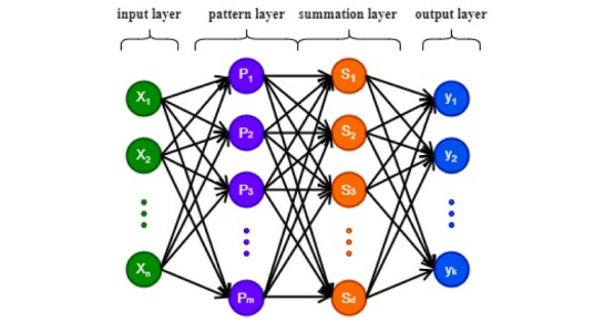
Neural Network Regression is a machine learning technique that uses an artificial neural network (ANN) to create a regression model for predicting continuous numerical values. The ANN learns from input-output data pairs, adjusting its weights and biases to approximate the relationship between the input variables and the target variable. This makes neural networks useful for predictive and forecasting applications.

Neural network regression is a supervised learning method that’s well-suited for problems where a traditional regression model can’t find a solution. It requires a tagged dataset with a label column that’s a numerical data type. The input features can be categorical or numeric, but the dependent variable must be numeric. If the output variable is categorical or binary, the ANN will act as a classifier.

Support Vector Regression (SVR)
Support Vector Regression (SVR) is a machine learning technique that uses Support Vector Machines (SVMs) to predict continuous numeric values. It’s an extension of SVM, which is mainly used for classification tasks. SVR is useful for regression tasks where linear regression may not be sufficient, such as when data has complex relationships or non-linear patterns.

SVR’s goal is to find a function that predicts a target variable while maximizing the margin between the predicted values and the actual data points. It does this by identifying a “margin” around the predicted regression line and fitting the line within that margin while minimizing prediction error. SVR uses an ε-insensitive loss function to penalize predictions that are farther from the desired output, and the width of the tube is determined by the value of ε. SVR also assigns zero prediction error to points that lie inside the ε-insensitive tube, and penalizes slack variables proportionally to their ξ. This feature helps SVR handle overfitting more effectively than other regression models.

SVR has several advantages, including: Robustness to outliers, Easy-to-update decision model, Excellent generalization capability, High prediction accuracy, and Easy implementation.

SVR’s ability to handle both linear and non-linear data makes it a versatile tool for a variety of real-world applications, such as financial forecasting, stock price prediction, economics, and engineering.

NN vs. Random Forest

When applied to somewhat limited data set availability, Random Forest machine learning techniques out-perform neural networks. Compared to a neural network, a random forest model generally offers advantages in terms of interpretability, ease of use, faster training time, and better performance with smaller datasets, making it a preferred choice when understanding feature contributions and working with limited data is crucial, while neural networks often excel in complex pattern recognition with large datasets where interpretability is less critical.

Key advantages of Random Forest over Neural Networks:

Interpretability:

Random forests are inherently more interpretable as you can easily examine the decision rules within each tree to understand which features are most important for predictions, while neural networks often function as “black boxes” with less clear feature relationships.

Data Requirements:

Random forests can perform well with smaller datasets, whereas neural networks typically require significantly more data to train effectively and avoid overfitting.

Training Speed:

Random forests generally train much faster than neural networks, especially on large datasets, due to their simpler structure and less complex computations.Random forests generally train much faster than neural networks, especially on large datasets, due to their simpler structure and less complex computations.

Less Preprocessing:

Random forests often require less data preprocessing compared to neural networks, which may need extensive feature engineering to optimize performance.

Robustness to Outliers:

Random forests are generally more robust to outliers in data compared to neural networks.

How AI “learns” to perform tasks

Artificial intelligence (AI) learns from data through machine learning algorithms that analyze data for patterns and correlations to make predictions or categorize information. The process of AI learning involves several steps, including:

Data collection and preparation:
Data is gathered from various sources, such as text, audio, and video, and then sorted into categories. The data is then processed and cleaned to prepare it for training.

Model and algorithm selection:
The right model and algorithm are chosen based on the type of problem, available data, and expected performance.

Training:
The algorithm is trained on labeled or unlabeled data to learn and grow.

Task completion:
The algorithm uses the training data to complete its tasks.

AI systems adapt through continuous learning and can take in new data to change and refine their process and outcome.

Note that the AI developer has control of what they desire the AI to learn and what its outputs should be. In the case of prostate AI, these range from very basic display-only functions to the heavy lifting of actual cancer detection and diagnosis.

In the case of Prostate AI trained for cancer detection, data for learning includes: prostate MRI data sets, accurately placed biopsy needle placement locations in 3D within the organ (using in-bore MRI guidance or FUSION guidance), and their resulting pathology reports. These data were then further processed by experts who hand drew (segmented) the organ perimeters on the images as well segmented the margins of the lesions surrounding the positive biopsy needle locations – these done by radiographic interpretation of the common features of the MRI associated with those biopsy needle locations.

The processed image data is then fed into the AI algorithm wherein the machine learning adapts its neural net or random forest weighting to optimize its own output to most closely mimic the true outcome recorded by the localized biopsy needle data (ground truth data).

Performance is measured according to how well the machine can then predict the outcome from images where ground truth is recorded but unknown to the machine. See “Variance in measuring outcomes” below.

AI in Prostate Cancer Detection, Diagnosis and Treatment Planning

Today’s Standard of Care (SOC), its limitations and its evolution

The following excerpt is from Improving standard of Prostate Cancer Diagnosis and Care is possible today with the use of non-contrast MRI and AI authored by Dr. Randall W. Jones, D.E. (PhD, MBA), printed in DotMed News June 2024. Prostate SOC is established via the NCCN (Vers. 2, 2024, 03/06/2024) Guidelines for Prostate Cancer Early Detection, and guidelines such as these typically lag behind the scientific and technical advancements by many years. In the interest of brevity, this 74 page guide is summarized herein. There are five basic steps involved: Baseline Evaluation, Risk Assessment, Early Detection Evaluation, Further Evaluation and Indications for Biopsy, and Management.

Baseline Evaluation involves reviewing the patient’s family history, environmental exposure, medications, race, and cancer history. Following the guideline’s flow chart, they recommend that the patient should undergo genetic testing if there is any family or personal history of high-risk germline mutations such as suspected cancer susceptibility genes (BRCA2, BRCA1, ATM, etc.). Continuing along the flowchart to Risk Assessment, regardless of the genetic testing outcome, if family history is concerning, shared decision-making is recommended regarding the timing and frequency of PSA testing. And further, regardless of that discussion, the flowchart indicates which risk category one should be placed in, average or high, and regardless of the risk category, the patient will eventually end up in the next step of Early Detection Evaluation if symptoms or suspicions persist.

STEP 3 NCCN guidelines: Early detection evaluation. In this step there is full reliance upon PSA and/or DRE taken at recommended intervals based upon risk category and age. For those patients with average risk and PSA<1 ng/ml and normal DRE (if done), repeat PSA and/or DRE at 2-4 intervals. Logical; however, for patients of average or high risk but with PSA,= 3ng/mL and DRE normal (if done), then repeat same tests at 1-2 year intervals. For those less than 75 years of age, if PSA>3 ng/ml and/or a VERY suspicious DRE; OR those greater than 75 and PSA>=4 ng/ml OR VERY suspicious DRE, then further evaluation is indicated for biopsy.
So in the end of these processes, the added cost of genetic testing and/or office visits has placed the patient in average or high risk categories based largely upon age and history/gene mutations, and suggests either monitoring with PSA and/or DRE OR if warranted, Advance to STEP 4, Further Evaluation and Indications for Biopsy.
PAUSE: In this guideline, there remains complete reliance upon PSA tests and DREs for early detection evaluation despite the facts that neither, nor their combination has a sensitivity-specificity much greater than 50%.

What if the above screening tests don’t reveal a cancer? The NCCN is recommending waiting another 1-2 years. Imagine the number of cancers left growing in this time-frame, and imagine that there was a better screening method.

STEP 4 NCCN guidelines: After repeat PSAs, DREs, then consider mpMRI or biomarkers that “improve the specificity of screening” such as Select MDx, 4Kscore, ExoDx, etc. prostate tests.

PAUSE: Regarding these biomarkers – they are very expensive. Who’s paying and at what benefit? Let’s focus on the benefit. In general these tests reveal a statistical score based upon one’s having PCa or susceptibility to having PCa. Even if the score is suggestive of prostate cancer, the next step is to get an MRI “if available” and/or proceed with an image-guided biopsy. Here’s the fine print on page 9 of the guidelines. “It is not yet known how such tests could be applied in optimal combination with MRI.”

STEP 4 concludes with STEP 5, Management: After the MRI or other biomarker, the patient is now considered either high or low suspicion for clinically significant prostate cancer (CSPC). The low risk classification leads to periodic follow-up using PSA/DREs again. If high, image-guided biopsy or transperineal approach with MRI targeting or without MRI targeting. Another words, they place no standard on the biopsy technic despite the published rather poor results of non-targeted standard 12 and 20 core biopsies.

DISCUSSION:
The above illustrates a number of fallacies and significant waste of medical resources and time. It is now well established that PSA is useful only in adding to the confidence of diagnosing cancer with the PSA density having some positive correlation to PCa; however, one has to have an accurate measurement of the organ volume and that also presents challenges and huge variations in accuracy amongst physicians performing manual measurements via MRI. DRE is only useful when a significant lesion is located in the posterior aspect of the gland; hence, nearly all anterior lesions are missed. Yet, the guideline heavily relies upon these antiquated non-specific, non-sensitive screening tests to guide a patient through early detection and diagnosis.

The argument about a better biomarker has been resolved. MRI plus a proven Detection and Diagnostic AI software can not only provide sensitivity-specificity results in the mid-90th percentile (Standalone AUROC that created physician improvement noted in this reference) [2], but also establish location, size, and classification of the suspicious lesion(s), in addition to the accurate volume of the gland – this without additional data such as the serum PSA or the expensive genetic tests or biomarkers.
The desired results of Prostate Cancer diagnoses are to have more definitive/accurate and early detections and/or confidence that the patient is cancer free. Moving the needle towards attaining these goals is the role of Artificial Intelligence in MRI interpretations.

How Imaging alone is improving outcome

Today’s Standard of Care (SOC), its limitations and its evolution

The following excerpt from An Overview of Current Clinical Studies of Prostate Cancer (PCa) Detection, Validation, Surveillance, and Treatment Options – Justification for MRI PCa Screeningauthored by Dr. Randall W. Jones D.E. (PhD, MBA). Whole article contained withing BotImage Inc. website www.botimageai.com.

MRI, and particularly multi-parametric MRI (mpMRI) has been widely published in recent years as THE biomarker for PCa. From an overview of several years of recent European peer-reviewed literature published over one year ago, “Multi-parametric magnetic resonance imaging is an emerging imaging modality for diagnosis, staging, characterization, and treatment planning of prostate cancer….There is accumulating evidence suggesting a high accuracy of mpMRI in ruling out clinically significant disease. Although definition for clinically significant disease widely varies, the negative predictive value (NPV) is very high at up to 98%.” Translation: if MRI does not detect clinically significant cancer, then one is assured at 98% confidence that they don’t have significant cancer!

The European studies have been mirrored by many in the USA. This from a leading researcher, Dr. Dan Margolis, at UCLA: “MRI can identify most men who would not benefit from biopsy, and can identify the index lesion in most men who would.” Based upon an extensive literature review and presented in June 2015, this was the overview of the standard of care at the time.
P hysical exam (DRE) + serum analysis (PSA)

•If either are abnormal → systematic biopsies
* >1M American men annually have an elevated PSA but negative biopsies
* False negative rate up to 47% depending on series
•Also risk of “over diagnosis:” assuming low grade disease on biopsy belies hidden aggressive cancer
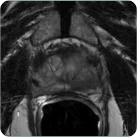
PI-RADSTM overview: The American College of Radiology (ACR) scoring system for interpreting mpMRI of prostate cancer.

In 2007 the AdMeTech foundation organized the International Prostate MRI Working Group, which brought together key leaders of academic research and industry for the purpose of addressing critical impediments to the widespread acceptance and use of MRI in diagnosing prostate cancer. They identified the excessive variation in the performance, interpretation, and reporting of prostate MRI exams, and resolved to bring additional standardization and consistency in order to facilitate multi-center clinical evaluation and implementation.

PI-RADSTM (Prostate Imaging and Reporting and Data System) version 1 was drafted in 2012 by the European Society of Urogenital Radiology (ESUR) to respond to the Working Group’s recommendations, and has since been validated in certain clinical and research scenarios.

The ACR, in conjunction with the ESUR and the AdMeTech Foundation, recently (late 2015) released PI-RADSTM v2 to address limitations of the earlier guidelines resulting from rapid progress in the field. The Steering Committee formed from this coalition consists of several working groups with international representation used the best available evidence and expert consensus from around the world.

In short, PI-RADS is a 5-point assessment scale based up the probability that a combination of mpMRI findings correlates with the presence of a clinically significant cancer for each lesion in the prostate gland. Clinically significant cancer is defined on the pathology/histology of Gleason score ≥ 7 (3+4, with the Gleason 3 being the predominant component), and/or volume ≥ 0.5cc, and /or extra prostatic extension (EPE).

PI-RADS Assessment Categories: Likelihood for presence of clinically significant cancer

  1. Very Low (Highly unlikely)
  2. Low (Unlikely)
  3. Intermediate (Equivocal)
  4. High (Likely)
  5. Very High (Highly likely)

Types of Imaging

MpMRI vs BpMRI

Multiparametric MRI (mpMRI) involves the added sequence of dynamic contrast enhanced (DCE) imaging which utilizes a tissue contrast agent, gadolinium, which allows for the assessment of tumor vascularization and necrosis, thus serving as a useful method for help in identifying cancerous tissues. Bi-parametric MRI (bpMRI) utilizes the same MRI acquisition sequences as does mpMRI except omits the use of contrast agents; thus, saving significant MRI system and operator time, cost of the expensive contrast agent, and most significantly, eliminates the potential harm done to kidneys – especially in compromised patients.
bpMRI has been shown to demonstrate almost perfect equivalence in detection accuracy as mpMRI when the MRI sets are read by experienced interpreters. However, a only a minority of physicians (radiologists) reading prostate MRI have accumulated the experience, through robust feedback of biological sampling (biopsies), to reach a proficiency of over 70% accuracy.

MRI in general has demonstrated sensitivity and specificity of 70-93% and 41-88% respectively in detecting clinically significant cancer. This wide range of performance is based upon many factors such as:

  • The region of the prostate where the cancer resides;
  • The size and significance of the cancerous lesions;
  • The quality of the MR image based upon MRI antenna (coil), magnetic field strength, DCE application, and most importantly the reader and his/her years and level of experience;
  • And the methods used in evaluation or measurement of performance.

Sensitivity is the ratio of true positives to true positives plus false negatives. Specificity is the ratio of true negatives to true negatives plus false positives.

Ultrasound

Ultrasound (US) works by sending high-frequency sound waves into the body and recording the echoes that bounce back. The echoes are used to create two-dimensional images of the body’s tissues and organs. Unfortunately, even the most advanced US, multiparametric or contrast enhanced US, has not demonstrated the sensitivity/specificity (in the 60th % range) to match even that of bpMRI.

However, the far less expensive US systems widely employed in urology clinics do create excellent anatomical images of the prostate in real-time such that the treating physician can cognitively hit targets provided by MRIs of the same patient.

FUSION Imaging

Certain Fusion System manufactures have created systems to “fuse” or overlay previous MRIs with real-time US images such that one can take advantage of the superior MRI lesion detection and with the overlay of the US image, then guide the biopsy or treatment probe into the targe lesion with a higher degree of accuracy.

PET/PSMA

A Prostate-specific membrane antigen positron emission tomography (PSMA-PET) scan is an imaging test that uses a radioactive tracer to detect prostate cancer throughout the body. The tracer binds to a protein called prostate-specific membrane antigen (PSMA), which is often found in high amounts on prostate cancer cells. The PET scan then detects the concentrated tracer to pinpoint the tumors.

PSMA-PET has high sensitivity and specificity for prostate cancer imaging:

  • Sensitivity: PSMA-PET has a sensitivity of 68.3% to 85%
  • Specificity: PSMA-PET has a specificity of 94% to 99.1%
  • Accuracy: PSMA-PET has an accuracy of 92% to 95.2%

PSMA-PET is more accurate than conventional imaging for initial prostate cancer staging. It can also be used to:

  • Detect malignant lesions in the prostate
  • Plan radiation therapy and surgery
  • Detect tumor recurrence, especially in patients with low PSA levels v

Here’s how a PSMA PET scan works:
A technician injects a radioactive tracer into a vein in the patient’s arm.

  1. The patient waits an hour for the tracer to be absorbed by the body.
  2. The patient lies down on a table that slides into a donut-shaped PET scanner.
  3. The scan takes about 30 minutes.

A doctor may order a PSMA PET scan to: Find cancer cells, Plan cancer treatment, and Check if cancer treatment is working.
A PSMA PET scan can be more accurate than other imaging tests for prostate cancer. It can also find very small tumors better than standard tests. However, these systems are quite expensive and installed in only the larger hospital systems so access is an issue for the general population.

Variance in measuring outcome – physician and AI performance

As mentioned above, measuring performance of physicians and AI varies and can significantly influence the reported outcomes. The following excerpt is from Current Problems in Diagnostic Radiology (Article in Press), Part I: prostate cancer detection, artificial intelligence for prostate cancer and how we measure diagnostic performance: a comprehensive review; Jeffrey H. Maki a,*, Nayana U Patelb, Ethan J Ulrichc, Jasser Dhaouadic, Randall W Jonesc
a. University of Colorado Anschutz Medical Center, Department of Radiology, 12401 E 17th Ave (MS L954), Aurora, Colorado, USA b. University of New Mexico Department of Radiology, Albuquerque, NM, USA c. BOT IMAGE Inc., Omaha, Nebraska, USA

Measuring performance in prostate cancer detection and diagnosis

Measuring performance in prostate cancer detection and diagnosis
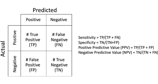
The literature is rife with different metrics for describing the performance of radiologists or AI algorithms in diagnosing prostate cancer, and it is important to understand how these are generated and what their limitations are. The most basic assessment as applied to the binary question of “is there cancer” defines “diagnosis”, which is at the case level. This can be assessed based on the confusion matrix (Fig. 1), a 2 × 2 table with the number of actual positive and actual negative cases on one axis, and the number of predicted positive and predicted negative cases on the other axis. As can be seen, the four boxes then contain the number of true positives (TP), true negatives (TN), false positives (FP) and false negatives (FN). From this, the standard statistical measures of sensitivity (or true positive rate), which is the TP divided by all positives = TP/(TP+ FN), and specificity (or true negative rate), which is the TN divided by all negatives = TN/(TN+FP), can be calculated. Many studies report sensitivity and specificity results for their readers or their AI algorithms, and in general a “good” reader or AI algorithm has a combination of high sensitivity and high specificity. Other metrics, such as positive and negative predictive value (PPV, NPV) are also often reported in studies, again derived from the confusion matrix, with PPV being TP divided by all those called positive = TP/(TP + FP) and NPV being TN divided by all those called negative = TN/(TN + FN).

Fig. 1. Confusion Matrix and the definitions for sensitivity, specificity, positive and negative predictive value.
ROC analyses
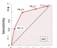
Applying such metrics may seem straight-forward, however there are numerous nuances to consider. First, how do we make the binary decision “positive” or “negative”? In fact, PI-RADS does NOT make such a decision as it is basically a five-point scale describing the likelihood of the patient having csPCa. Assume for a moment we call only PIRADS 5 lesions “positive”. Provided we have ground truth (e.g. biopsy, explant pathology), we can then calculate sensitivity and specificity. Alternatively, we could choose to call PIRADS ≥ 4 lesions positive, yielding a different sensitivity and specificity, and so on for PIRADS ≥ 3 lesions and
≥ 2 lesions. By doing this, we arrive at four different sensitivities and specificities corresponding to the different PIRADS thresholds. These values can be plotted on a Receiver Operating Characteristic curve (ROC), with the x axis (1 – Specificity) and the y axis Sensitivity, as shown for hypothetical data in Fig. 2. Note that by calling all PIRADS ≥ 2 positive our sensitivity is very high, but at the price of low specificity. Conversely by only calling PIRADS 5 lesions positive, our specificity is high, but our sensitivity suffers. The diagonal line is known as the line of “no discrimination”, i.e. purely random; points to the left of this line are better than random, and points to the right worse than random, with top left (0,1) being perfect. With AI, there may be a more continuous vari- able characterizing the probability of prostate cancer, for example a continuous probability ranging from 0 to 1. Under these circumstances, many more points can be generated to fill-in the ROC curve such that it is smoother and can help to choose the optimum threshold given the desired outcome, or compare between different readers/techniques. A useful and often used numerical measurement of performance well suited to comparison is the “area under the (ROC) curve”, or AUC, illustrated as the shaded area in Fig. 2, which ranges from 0≥ 2 lesions. By doing this, we arrive at four different sensitivities and specificities corresponding to the different PIRADS thresholds. These values can be plotted on a Receiver Operating Characteristic curve (ROC), with the x axis (1 – Specificity) and the y axis Sensitivity, as shown for hypothetical data in Fig. 2. Note that by calling all PIRADS ≥ 2 positive our sensitivity is very high, but at the price of low specificity. Conversely by only calling PIRADS 5 lesions positive, our specificity is high, but our sensitivity suffers. The diagonal line is known as the line of “no discrimination”, i.e. purely random; points to the left of this line are better than random, and points to the right worse than random, with top left (0,1) being perfect. With AI, there may be a more continuous vari- able characterizing the probability of prostate cancer, for example a continuous probability ranging from 0 to 1. Under these circumstances, many more points can be generated to fill-in the ROC curve such that it is smoother and can help to choose the optimum threshold given the desired outcome, or compare between different readers/techniques. A useful and often used numerical measurement of performance well suited to comparison is the “area under the (ROC) curve”, or AUC, illustrated as the shaded area in Fig. 2, which ranges from 0
ROC Curve

1 –Specificity (False Positive Rate)

Fig. 2. Hypothetical example of Receiver Operating Charateristic (ROC) curve. Area under the curve (AUC) represented by red shading.
to 1. AUC provides a more global picture of performance across differing thresh- olds. A perfect score would be 1.0, and the literature often describes prostate AI achieving AUC > 0.9; however, we will further discuss how these values are significantly influenced by the exact mechanism by which the ROC/AUCs were measured; meaning that the AUC values reported cannot be directly compared unless the exact methods are also shared and identical.
PCA case level vs. lesion level diagnosis
Another important consideration when examining how radiologists or algorithms perform has to do with how we define what constitutes a “correct” diagnosis? Considering only a single diagnosis for the case (case level diagnosis), calling a malignant lesion somewhere in the prostate is considered “correct” even if the identified lesion is a false positive and the true malignant lesion is totally missed. On the other hand, we could score each identified lesion individually and use this to determine our performance (lesion level diagnosis). How we chose to do our evaluation has the potential to become even more problematic with AI, which may perform the analysis on a pixel-by-pixel level. Should we somehow try to do the analysis of truth pixel-by-pixel (and is that even possible given what we have for truth?). Do we consider only the highest probability pixel in a “suspicious” region? Or a cluster of higher prob- abilities of a certain size? These are all different approaches that will lead to different results.
Establishing ground truth and scoring system
All of this introductory information has been provided as back- ground for how to evaluate and analyze a comparative study of radiol- ogists performing PIRADS reads with and without the help of a prostate CADe/CADx system. Given all of the variables discussed, it is clear that one must establish a solid clinical study so as to minimize measurement errors and follow a common standard. We believe the radiology com- munity thus far lacks such guidance that standardizes the methodologies for:

  • Measuring a non-continuous diagnostic system such as PI-RADS
  • Generating ROC curves with fixed numbers of evaluation points (pixels, 3D grids, PI-RADS sub-regions, etc.)
  • Determining how to evaluate reader and software detection of le- sions and defining what is truly a “hit” versus “miss” of a lesion based upon the granularity of division of the prostate, or “how you slice it”
  • How best to ethically establish and accurately place three- dimensional pathology ground truth points or volumes within the three-dimensional MRI data set
  • And perhaps most challenging of all, how to establish whether non- suspicious (unsampled) tissues and patient cases are truly negative for cancer
  • Although the FDA provides guidance documents on Clinical Performance Assessment of CAD radiologic software, as well as guidance on establishing clinicals studies for Computer-assisted Detection Devices Applied to Radiology Images, the detailed methods outlined above are left to the submitting medical device companies. It is therefore highly unlikely that any two radiological CAD devices or peer-reviewed papers discussing the performance of a device can be directly compared because of the significantly different outcomes resulting from the non-standardization of the above methods and procedures.

Types of AI and influence on detection, diagnosis and treatment planning

There are many different levels of AI in terms of the functions offered by the algorithm; hence, the user must beware of those functions and their limitations. For instance, on the low end of AI, there are display software algorithms that conveniently display the various series of prostate MRI including a graph of the DCE uptake and outflow over time in a given suspect area as identified by the radiologist. These programs may also perform a draft segmentation of the prostate organ and facilitate the physician’s proofing and agreement. No learned AI function of lesion detection or diagnosis is provided. In the middle range of functions, some algorithms automatically perform organ segmentation and even point to suspect areas without segmenting of classifying these areas. The later with full automation of the organ segmentation represents the high end of AI functionality.
Note that the types of AI machines also have an impact upon the detection performance as indicated in “Performance Comparisons…” below.

Variations in AI systems based upon Installation

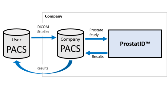
Electronic data connection between the MRI system and the AI software is obviously necessary in order to feed the software with MRI studies and obtain the resulting outputs. These connections can come via three different methods:

  • direct secure VPN tunnel of PACS or MRI System to the AI provider’s PACS;

  • connection from the user’s PACS or MRI System to a third-party AI Platform typically installed behind the hospital of MRI facility’s firewall;
  • connection from the PACS or MRI System to a separate stand-alone computer system containing the provider’s AI.

Components of working AI systems (how they work)

This paper has described the various detection models, also referred to as “inference models”; however, many other steps must be taken to ensure safety, security and efficacy of the software, not to mention, consistent operation.
As an example, the ProstatID® (Bot Image, Inc., Omaha, NE) software algorithm consists of six functional steps as indicated in the Architecture Design Chart (Figure below), and summarized below.

  • Automatic Detection of Prostate Input Images.
  • Image quality testing for Complete Study of 3 series, three complete series of equivalent total slice volume, minimum resolution.
  • Prostate segmentation, feature calculation and cancer classification
  • CAD Report Generation.
  • Return DICOM outputs to Users
  • Delete Study

Automatic Detection of Prostate Image Inputs

ProstatID continually queries the PACS server for new prostate studies and automatically begins processing after a new study arrives. The software searches the DICOM image data to determine the relevant prostate study and image series needed for processing.

Image Quality Testing

The image quality function tests to ensure that the image quality meets minimum requirements prior to processing. This functional test consists of checking to ensure that the three axial image series are: i) present, ii) tested to ensure that each series contains the total slice volume (i.e., that the number of slices plus slice gaps times their widths) are equivalent, and iii) meet the resolution quality required by the software which tracks with PI-RADS recommendations.

Prostate Segmentation, Registration, Feature calculation and Cancer Classification

After performing a quality check on its input, the software is designed to preprocess the approved medical data before making any cancer prediction.
ProstatID automatically detects the anatomy of the prostate in the T2-weighted MR image of the male pelvic region. Classification is accomplished by utilizing an ensemble modelling approach where various base models are used during the process of cancer prediction (further explained in the section below).

CAD Report Generation of Algorithm Output

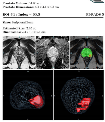
After creation of the color overlay in Function 3, the algorithm proceeds to generate the report (Figure below) consisting of the colorized probability map, correlated to classification of cancerous tissue, overlaid on a copy of the T2-wieghted image set, and a 3D rendition of each suspect lesion with probability greater than 62%.

Return DICOM outputs to Users

All outputs are formatted to be DICOM-compliant. The encapsulated PDF report and the post-processed T2-weighted colorized series is then automatically returned via the same connection to the sender’s radiological workstation indicating a unique post-processed series number which appends to the original patient study via the unique study number for the physician to identify as such.

Delete Study

The study is deleted from the local PACS upon either a failed study from quality testing (Function 2) or upon a successful study and confirmed returned output (Function 5) to the user’s PACS.

Refined Random Forest – Boosted Parallel Random Forest

A novel boosted parallel Random Forest model was created (Bot Image, Inc., Omaha, NE) by building upon a successful prototype developed by researchers at the NIH (National Institutes of Health, Bethesda, Maryland) wherein 64 “features” extracted from three MRI series, T2W axial, DWI and ADC were used as inputs to the detection algorithm. Most of these features are non-detectable to the trained human eye; however, the prove useful in distinguishing tissue types from the MRI image sets and provide improved detection and cancer classification power over trained readers.

Bot Image’s model 64 input features and 3 outputs: lesion detection, segmentation and classification.

The figure below is a schematic of Bot Image’s boosted parallel random forest (bpRF) model architecture. bpRF is an ensemble of various base models. The ensemble model seeks the wisdom of the crowd and aggregates the prediction of each base model to make a final prediction with less generalization error. bpRF implements a chain of estimators that starts with an AdaBoost7 model encapsulating multiple bagging classifiers that are boosted sequentially during training. Each bagging classifier8 has 5 parallel random forests acting on random slices of data.

Performance Comparisons of Boosted Parallel Random Forest, NN, Standard Random Forest and others in PCa detection – ISMRM

A test comparing the performance of trained models of prostate cancer detection models using different types of machine learning was conducted and reported in an academic paper presented at the International Society of Magnetic Resonance in Medicine, Annual meeting 7-12 May 2022, London, UK.

Comparison of machine learning methods for detection of prostate cancer using bpMRI radiomics features Ethan J Ulrich1, Jasser Dhaouadi1, Robben Schat2, Benjamin Spilseth2, and Randall Jones1; 1Bot Image, Omaha, NE, United States, 2Radiology, University of Minnesota, Minneapolis, MN, United States

The following are excerpts from the paper above which can be viewed within the ISMRM Book of Abstracts.

Synopsis

Multiple prostate cancer detection AI models—including random forest, neural network, XGBoost, and a novel boosted parallel random forest (bpRF)—are trained and tested using radiomics features from 958 bi-parametric MRI (bpMRI) studies from 5 different MRI platforms. After data preprocessing—consisting of prostate segmentation, registration, and intensity normalization—radiomic features are extracted from the images at the pixel level. The AI models are evaluated using 5-fold cross-validation for their ability to detect and classify cancerous prostate lesions. The free-response ROC (FROC) analysis demonstrates the superior performance of the bpRF model at detecting prostate cancer and reducing false positives.

Results

The bpRF model, which extracts intensity and texture features for detecting prostate cancer based upon Lay’s model from the NIH, outperforms other machine learning methods (random forest, UCLA’s neural network, and XGboost – a gradient boosting machine) as demonstrated by an improved FROC performance indicating fewer false positives and false negatives. Additionally, the algorithm has demonstrated the potential of more accurately depicting the actual size and outline of the cancerous lesions.

The performance metric for FROC is the weighted alternative FROC (wAFROC) figure of merit and is analogous to the ROC AUC. The bpRF model (from ProstatID of Bot Image, Inc., Omaha, NE) had significantly higher performance when compared to NN (p=0.007), RF (p=0.003), and XG (p=0.002) after adjusting for multiple comparisons.

Detections are evaluated at each biopsy location and local maxima within the predicted probability map. False positives are defined as detections at biopsy sites with combined Gleason score < 7 or a local maximum that is more than 6 mm from a known lesion. Curves and the performance metric (θ) are the average of the cross-validation folds. NN = neural net, XG = XGBoost, RF = random forest, bpRF = boosted parallel random forest.

Discussion

While all models demonstrated similar performance when evaluating at the lesion-level (ROC analysis), bpRF outperforms other models on FROC analysis. This indicates that the bpRF model produced fewer false positive detections at equal sensitivity.

Image Guided Treatment Systems

A number of manufacturers, Koelis®, Eigen Health, GE Healthcare, Siemens Healthineers, and others, have created systems that combine MRI results with real-time ultrasound (US) images of the same patient; thereby taking advantage of the superior sensitivity/specificity of MRI to combine with the ultrasound while in a urology treatment room and eliminating the use of expensive MRI time for treatment guidance.

These systems utilize the lesion identification assistance of AI powered MRI to provide targeting for needle and treatment probe placement while combining or fusing the MRI images to real-time US images and viewing the needle/probe placement on a computer screen to ensure placement within the MRI targets.
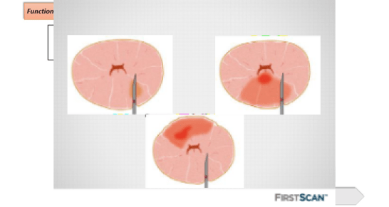
 

The Challenge of Needle biopsy

Obviously, the quality of the AI powered MRI has a significant effect on the outcome of the biopsies and/or treatments. For instance, if the AI or lack thereof, has not accurately identified the cancerous targets, then those biopsies and/or treatments will be ineffective. Therefore, it is imperative that physicians chose the systems incorporating the most advanced MRI detection algorithms.

AI in Post-Treatment and/or Active Surveillance

SOC PCa End Game: Treatment Options (typically)

  • Do nothing
  • Prescribe antibiotic
  • Radical prostatectomy
  • Brachytherapy
  • Hormone Therapy
  • HIFU

For sake of brevity, we leave it to the reader to review the benefits, risks and side effects of the various options above with their physician as they vary considerably.
Our message is that all cancers are not the same; therefore, one treatment does not fit all. Often, an antibiotic regiment will dissipate symptoms such as rising PSA, frequent urination, and others due to simple prostatitis infection in the gland.

Also, it has been well studied1 and documented that often doing nothing and actively monitoring (via periodic PSA measurements and/or repeat MRIs) is better than the more radical treatments (surgery and therapies) above. This is based upon the age, symptoms, health, and emotional condition of the patient.

  1. Hamdy, Donovan, Lane, Metcalfe, et. al., Fifteen-year Outcomes after Monitoring, Surgery, or Radiotherapy for Prostate Cancer, NEJM, March 11, 2023. DOI: 10.1056/NEJMoa2214122

For AI to be effective in detecting cancer in post-treated patients, the AI must be “trained” with the same type of ground truth data as it was trained with untreated patients. This includes the MRI study, 3D biopsy needle placements and corresponding pathology reports.
The FDA and other regulatory bodies tightly regulate the labeling and use of software as a medical device and therefore the manufacturers must clearly spell out the Indications for Use and describe what patients are not indicated for using the software potentially such as post-treated patients.

AI in Pathology Interpretation

The latest use of AI is in pathology interpretation. Slides of prostate pathology have been used to train computer models to recognize various stages of cancerous cells within microscopic cellular mounts.
Again, the pertinent issues affecting clinical outcome are:

  • What guidance, if any, was used to target the biopsies?
  • How did the interventionalist know that he/she hit the target?
  • How were the biopsies taken and how large of samples?
  • How accurate was the method used?
  • How experienced was the pathologist in interpreting cellular mounts?

The literature has demonstrated the effectiveness of AI used in interpreting and classifying cellular slide pathology; hence, further improving the standard of care in prostate cancer detection and classification.

Remember, you can Insist on the best quality of care, and you are encouraged to seek other options to cancer diagnosis or surgeries, so learn about those options here and elsewhere.